Introduction

In this lesson, you will learn how to calculate the payment on a loan using the PMT function in Excel.

This video illustrates the lesson material below. Watching the video is optional.

• How to Calculate the Payment on a Loan (8:00 mins) | Transcript

Loan Payment Equation

Before looking at the PMT (payment) function in Excel, look at the calculating loan payment equation outside of Excel. This equation does not need to be memorized. It will simply aid in explanation and act as a reference.

\begin{align*} PMT=\frac{(Pv)\frac{annual\;rate}{n}}{1-(1+\frac{annual\;rate}{n})^{-nt}}\end{align*}

• Pv = The present value, or total amount of the loan.
• Annual rate = The annual interest rate.
• n = The number of times the interest rate will compound in a year.
• t = The number of years.

PMT Function in Excel

The payment function in Excel uses the following arguments: rate, nper, and pv. There are two other variables in this formula that are optional. This lesson will not focus on those.

• The rate is the annual rate divided by the number of times the interest compounds. This can also be called the periodic rate. 
• The nper is the \(^{-nt}\) in the equation, or the number times the interest compounds over the entire course of the loan. 
• The pv is the present value, or total amount of the loan at the start of the loan. 

You need to calculate the rate and nper before putting them into the payment function.

Example 1
Use the PMT function in Microsoft Excel to calculate the monthly payment Sally will need to pay for a loan on a car that is $19,000. The annual interest rate is 6%. The loan will last 5 years.

Start by typing important information in Excel. See Figure 1.

• Type Present Value in cell A1 and 19000 in cell B1.
• Type Annual Interest Rate in cell A2 and 6% in cell B2.
• Type Number of Years in cell A3 and 5 in cell B3.
• Type Payments per Year in cell A4 and 12 in cell B4.

Figure 1

Next, calculate the rate for the PMT function.

• Type Rate (periodic rate) into cell A6. In cell B6, use cell references to divide the Annual Interest Rate (in cell B2) by the Payments per Year (in cell B4). It will look like this: =B2/B4.

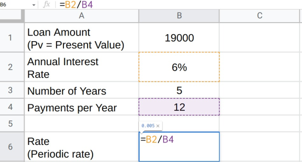
Figure 2

• Press Enter. The periodic rate should appear in cell B6. In this case, the rate is 0.005.

Next, calculate Sally’s loan nper, or the total number of payments.

• Type nper (number of payments) into cell A7. In cell B7, use cell references to multiply the Number of Years (in cell B3) by the Payments per Year (in cell B4). It will look like this: =B3*B4.

Figure 3

• Press Enter. The nper should appear in cell B7. In this case, the nper is 60.

Now you have everything you need to calculate the monthly payment using the PMT function in Excel.

• Choose a new cell and insert the equal sign (=), followed by PMT. Beneath the cell, a small box will appear. The box will tell you the order that you must put your arguments/variables in.
• The first argument is rate or periodic rate. Reference cell B6. Add a comma.
• The next argument is nper or the number of payments. Reference cell B7. Add a comma.
• The final argument is pv or loan amount present value. Reference cell B1. Close the parentheses.

Figure 4

• Press Enter. The answer should appear: -367.32.

The answer should show as a negative number. This is because this is a payment. If Sally pays this amount, she will lose $367.32 every month for the next 5 years. This amount includes the principle and the interest that she would pay each month on the loan.

Figure 5

Things to Remember

• It is helpful to use this equation as a reference: \(PMT=\frac{(Pv)\frac{annual rate}{n}}{1-(1+\frac{annual rate}{n})^{-nt}}\)
• To calculate a loan payment in Excel, you need to know the rate, nper, and the Pv or present value.

Practice Problems

1. Use Excel to calculate the monthly payment on a $45,000 loan for a small business with an interest rate of 7.5% over 10 years. (
   Solution

   x

   Solution: \($534.16\)
   
   Details:
   First you need to determine the following:
   
   Number of payments per year \(= n = 12\)
   
   Number of years \(= 10\)
   
   Annual rate \(= r = 0.075\) (or \(7.5\%\))
   
   Amount of loan \(= {\color{Red}Pv} = {\color{Red}45000}\) (Do not use commas in Excel except to separate each argument.)
   
   \(\displaystyle\text{Periodic Interest Rate}=\frac{\text{r}}{\text{n}}=\text{rate}=\frac{0.075}{12}\text{ or }\frac{7.5\%}{12}\)
   
   Total Number of Payments \(= {\color{Magenta}nper} =\) number of years \(\times\) payments per year \(= 10 \times 12 = {\color{Magenta}120}\)
   
   Open an Excel spreadsheet. Select a cell and type: =pmt(
   
   
   
   Excel will bring up a box with "PMT(rate, nper, pv, [fv], [type])" written in it to remind you what order to enter your arguments. Continue by entering the values for rate, nper, and pv. You don’t need to enter anything for fv or type—these arguments are optional.
   
   
   
   Then select Enter. Excel will then display the payment amount which is \($534.16\). Note that it is in red and has parentheses around it indicating that it is an expense.
   
   
   )
2. Use Excel to calculate a car payment compounded monthly given the following values: (
   Solution

   x

   Solution: \($222.14\)
   
   Details:
   First you need to determine the following:
   
   Number of payments per year \(= n = 12\)
   
   Number of years \(= 6\)
   
   Annual rate \(= r = 0.0575\) (or \(5.75\%\))
   
   Amount of loan \(= {\color{Red}Pv} = {\color{Red}13500}\) (Do not use commas in Excel except to separate each argument.)
   
   \(\displaystyle\text{Periodic Interest Rate}=\frac{\text{r}}{\text{n}}=\text{rate}=\frac{0.0575}{12}\text{ or }\frac{5.75\%}{12}\)
   
   Total Number of Payments \(= {\color{Magenta}nper} =\) number of years \(\times\) payments per year \(= 6 \times 12 = {\color{Magenta}72}\)
   
   Open an Excel spreadsheet. Select a cell and type: =pmt(
   
   
   
   Excel will bring up a box with "PMT(rate, nper, pv, [fv], [type])" written in it to remind you what order to enter your arguments. Continue by entering the values for rate, nper, and pv. You don’t need to enter anything for fv or type—these arguments are optional.
   
   
   
   Then select Enter. Excel will then display the payment amount which is $222.14. Note that it is in red and has parentheses around it indicating that it is an expense.
   
   
   )
   
   • Amount of loan = 13,500
   • Annual interest rate = 5.75%
   • Length of the loan = 6 years
3. Use Excel to calculate a house payment compounded monthly given the following values: (
   Solution

   x

   Solution: \($1154.43\)
   )
   
   • Amount of loan = 245,500
   • Annual interest rate = 3.875%
   • Length of the loan = 30 years
4. Use Excel to calculate the payment on a personal loan to a friend of $150 with an annual interest rate of 7% over six months (0.5 years) with the interest calculated monthly. (
   Solution

   x

   Solution: \($25.51\)
   )
5. Use Excel to calculate the payment on a credit card balance of $5000 with an annual interest rate of 19.99% over five years with the interest calculated monthly. (
   Solution

   x

   Solution: \($132.44\)
   )
6. Use Excel to calculate the monthly payment on an $800 cell phone at 5.25% interest over two years. (
   Solution

   x

   Solution: \($35.19\)
   )

Need More Help?

1. Study other Math Lessons in the Resource Center.
2. Visit the Online Tutoring Resources in the Resource Center.
3. Contact your Instructor.
4. If you still need help, Schedule a Tutor.