Introduction

Negative numbers have a different set of rules than positive numbers. In this lesson, you will learn how to handle negative numbers in Excel.

This video illustrates the lesson material below. Watching the video is optional.

• Negative Numbers in Excel (06:49 mins) | Transcript

Arithmetic with Negative Numbers

Negative numbers are represented in Excel with a hyphen (-) and a number. In Excel, you can reference cells with negative numbers just as you would positive numbers. You can also write equations with negative numbers as illustrated in Figure 1 and Figure 2.

Example 1

• In cell A1, type negative 8 (-8).
• In cell A2, type negative 4 (-4).
• In cell C1, type the equal sign followed by A1 plus A2 (=A1+A2).
• Press Enter to calculate the arithmetic equation.

Figure 1

Example 2

• In cell C2, type the equal sign followed by A1 star A2 (=A1*A2).
• Press Enter to calculate the multiplication equation.

Figure 2

Cell Formatting

There are many ways to show negative numbers in Excel. Cells can be formatted to display negative numbers in these different ways. Some of these notations are used in accounting, bookkeeping, and finance.

1. Right-click  on the cell you would like to format. Pick the Format Cells option. This will open the Format Cells panel.
2. In the Format Cells panel, select the Number option.
3. In the Number option, choose the Number category
4. In the Number option you will see four options for negative numbers:

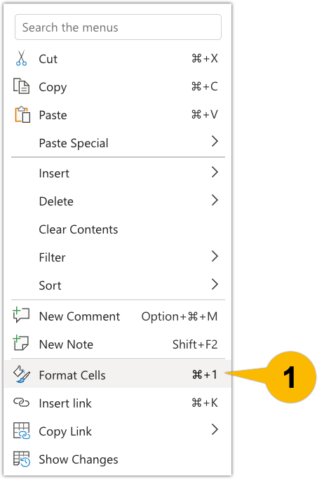
Figure 3

• \(-1234.10\): This option keeps negative numbers black with a negative symbol in front.
• \(\color{red}\mathbf 1234.10\): This option turns negative numbers red without a negative symbol.
• \((1234.10)\): This option keeps the negative number black but displays them within parentheses. This notation is often used in accounting and bookkeeping.
• \(\color{red}\mathbf (1234.10)\): This option turns negative numbers red and displays them within parentheses.

Note: This course will most often use the first option: black numbers with a negative symbol in front. This format is recommended for your coursework.

You can see cell A1 has been formatted to be a number cell. It is a negative black number with two decimal places. You can change this cell in the Format Cells panel.

Figure 4

Example 3
In Figure 5 there is a list of numbers. Notice there are both positive and negative numbers. Here are basic steps to format cells as currency in different ways:

1. Highlight the data you would like to format. Right-click and select the Format Cells. This will open the Format Cells panel.
2. In the Format Cells panel, select the Number option.
3. In the Number option, select Currency from the category list.
4. Select the symbol of currency that is being used.
5. Select the desired display option for negative money numbers. For this course, the first option is highly recommended, in which negative numbers are the same color as others and preceded by a hyphen.

Figure 5

Note: In the Number category, the negative number display options are the same, except they are displayed without a currency symbol.

For this example, select the second option where negative numbers turn red. All the negative numbers are in red and the positive numbers are in black. The problem with this option is that you risk forgetting the red numbers are negative.

Figure 6

Arithmetic problems using these numbers will function the same. To demonstrate, try adding one of the positive numbers and one of the negative numbers from the list above, as shown in Figure 7.

Example 3

• In cell D1, type the equal sign (=).
• Select cell B1, which contains a negative number.
• Type the plus sign (+).
• Select cell B6, which contains a positive number.
• Press Enter to calculate the arithmetic equation.

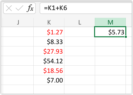
Figure 7

Arithmetic Equations with Negative Numbers

While it can be helpful in some instances, you do not need to format negative numbers. As another option, negative numbers can simply be typed into formulas. You can reference cells with negative numbers just as you would reference cells with positive numbers.

For example: If you type =-3*-5-1 into a cell and press Enter, you should see the number 14 appear in the cell, because of the order of operations: -3*-5 + -1 = 15 +-1 = 14.

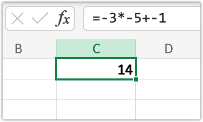
Figure 8

Note: You may want to use parentheses in examples like this to make them more readable, such as: =(-3)*(-5)+(-1). Excel will follow the order of operations.

Things to Remember

• If you want to reformat your cell, simply right-click the cell and select Format Cells….
• Parentheses are helpful when writing out equations that contain negative numbers.

Need More Help?

1. Study other Math Lessons in the Resource Center.
2. Visit the Online Tutoring Resources in the Resource Center.
3. Contact your Instructor.
4. If you still need help, Schedule a Tutor.